A Dynamical Simulation of Linked Rigid Body Systems using Impulse Technique

Abstract

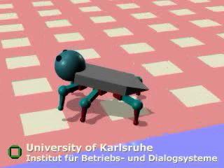
We present a new method for the dynamic simulation of linked rigid body systems. Forces are systematically substituted by impulses. In this way we succeed to perform the simulation in a very direct way and without solving complex systems of differential equations. The basic principle of the method is a new iterative procedure to calculate impulses which conserve joint constraints. The implementation of the method is comparably simple and it is very fast and accurate. This is documented by a first presentation of experimental data and accuracy estimates. In order to start the simulation, mechanical models need only minimal preprocessing. The impulse-based method is also very flexible if new types of joints have to be introduced. Collision and friction are implemented in a direct manner. The method is especially well suited for the new generation of VR systems with correct dynamical and kinematical behavior of VR-worlds. It is also well suited for the simulation of mechatronic systems since the simulation of complex models like six-legged walking machines is possible in real time on a PC.

View the Project Description        View the Animations

Project Description

The goal of the new impulse-based dynamic simulation method is to correctly simulate rigid bodies, also taking into consideration that rigid bodies can be connected by joints (e.g. hinge joints). On each of these joints, continuous forces are acting in order to keep the bodies together and these forces can be computed by solving complex differential equations. The designed dynamic simulation system should also be able to correctly simulate collision and friction.

How does the method work?

In the simulation method, continuous forces are simulated by impulses because in this way no complex differential equations have to be solved. According to Newton's second law, force equals mass times acceleration. Therefore, if a continuous force is integrated over a time interval, the result is the change of impulse.

Parameters necessary for the simulation:

The mass and the inertia tensor (in body space coordinates) are constant over time, in contrast to all the other parameters, which have to be updated after every simulation step.

A rigid body in the simulation is defined at time t by:

1. mass m_k

2. center of mass C_k(t)

3. velocity v_k(t)

4. inertia tensor J_k

5. rotation matrix R_k(t)

6. angular velocity w_k(t)

The position of the rigid body in the global coordinate system is well-defined by its center of mass and its rotation matrix.

How does the method work for rigid bodies connected by joints?

The simulation of single rigid bodies is relatively straight forward, however, this is more complicated when rigid bodies are connected by joints, where every joint is represented by a certain constraint. In order to be able to explain the method of simulation a ball joint will be used as an example. This kind of joint has 3 degrees of freedom and the constraint of the ball joint is that the distance between the two joint points must not be greater than a certain tolerance constant. We call a multibody system consistent if every constraint is satisfied.

In this picture we can see a ball joint and its constraint is satisfied

Here the joint is broken because the distance between the two joint points is greater than the tolerance value.

These joint constraints are really important because their inconsistency leads to the need to compute correction impulses that keep the joints together. The pictures below describe exactly this process of applying an impulse on two rigid bodies connected by a ball joint to form a  double pendulum. The effects that the impulse produces on the joint and the necessity of a correction impulse in order to keep the joint constraint are visualized.

time t
look ahead: t+h (without correction)	time t+h (with correction)

A(t) and B(t) mark the two points of the ball joint that have to be within a certain distance d_max so that the joint constraint is satisfied. At time t the constraint of the joint is still satisfied, however, if a simulation step is made without regarding the joint constraint, due to gravity the joint will be broken at time t+h, where h is the time step size. That is why it is necessary to compute a correction impulse p that will take into consideration the force of gravity and other forces that would be acting on the joint. The correction impulse works against the effect of these forces on the joint and in this way ensures its consistent state.
It is important to notice that in order to get a consistent system at time t+h, the correction impulse must be applied at time t. In this way, the impulse changes the velocities of the two rigid bodies and if the same simulation step is made again, it will result in a consistent system at time t+h.
In case of a system with more than one joint, correction impulses have to be computed for every joint and their updating after each application continues iteratively until all constraints are satisfied.
 

How is the correction impulse computed?

The difference between the velocity changes of the two joint points A(t) and B(t) must be equal to the distance vector d divided by the time step size h. That means that the impulse p will make the distance vector to zero at time t+h and the joint constraint will remain satisfied. In this way by using the described conditions, equations can be written and the correction impulse can be computed.

How is the correction impulse computed for more than one joint?

1) First, joint corrections have to be made for all joints. For each joint a position look ahead is made and it is checked if the constraint is satisfied at time t+h. If it is, it can be proceeded with the next joint. Otherwise, a correction impulse has to be computed and applied . The joint corrections are made in an iterative loop until all constraints are satisfied.

2) After all corrections are done the center of mass C_k(t), the velocity v_k(t), the rotation matrix R_k(t) and the angular velocity w_k(t) of all rigid bodies have to be updated. Then the positions of the joint points are updated because they are needed for the next simulation step.
3) The last part of a simulation step is a velocity correction. In general, after the first two parts of a simulation step, the velocities in the two points of a joint are not equal anymore. To correct this a similar method like for the joint correction can be used. First, the velocities of the joint points are computed. Then it is checked if the difference between the velocities is greater than a certain tolerance value. If it is greater, a correction impulse can be computed and applied so that the constraint will be satisfied. In this way, it can be proceeded with the velocity corrections in an iterative loop until all constraints are satisfied. The velocity corrections are not essential for a simulation, but they help to achieve better accuracy.

Example for a single joint correction

Pendulum This is video about a triple pendulum which illustrates the single joint corrections. Size:  7,7 MB Type: .mpeg

Results

Here are described some results for the simulation method.

• On a computer with 1.7 GHz we can make 670.000 joint corrections per second.
• The advantage of the iterative method is that the loop can be interrupted at any time to get a result.
• If the loop is interrupted there is a loss of accuracy. However, especially for virtual reality applications it is sometimes more important to get a result in real-time than to have a high accuracy.
• Also in the simulation there can occur some situations where the system can’t be corrected if the time step size is too large but this problem can be easily solved by using an adaptive time step size.
• Finally, the correction method can even fix a model which has totally broken joints.

Animations

• 8-loop: No collision detection and resolving used
• Sliding cubes: Each cube has a different friction coefficient
• A walking machine -on ice-
• A rotating egg
• A walking machine -escaping-

• A pendulum on a sledge 1
• A walking machine -toppling over-
• A pendulum on a sledge 2
• Pendulum

8-loop: No collision detection and resolving used A chain with 8 segments. Both ends of the chain are fixed, which creates a closed kinematic loop. Size:  1,6 MB Type: .mpeg

Sliding cubes: Each cube has a different friction coefficient This video compares the outcome of a simulation with analytically computed target positions for several friction coefficients. Size:  1,3 MB Type: .mpeg

A walking machine -on ice- A six-legged walking machine on a surface with a small friction coefficient (simulating ice). Size:  1,7 MB Type: .mpeg

A rotating egg This video shows a rotating "egg" that rises from a lying position to an upright position because of its rotation. Size:  7,8 MB Type: .mpeg

A walking machine -escaping- The walking machine manages to get to a surface with a higher friction coefficient where it's able to gain speed. Size:  3 MB Type: .mpeg

A pendulum on a sledge 1 A pendulum mounted on a sledge on an inclined plane with a relatively high friction coefficient. The sledge makes the typical "stop and go" movements. Size:  2,6 MB Type: .mpeg

A walking machine -toppling over- The walking machine lands on its back because it was pushing too hard with its leg. Size:  2,3 MB Type: .mpeg

A pendulum on a sledge 2 The same setup as before but this time with a small friction coefficient. Size:  1,1 MB Type: .mpeg

Pendulum This is video about a triple pendulum which illustrates the single joint corrections. Size:  7,7 MB Type: .mpeg

Links

Download